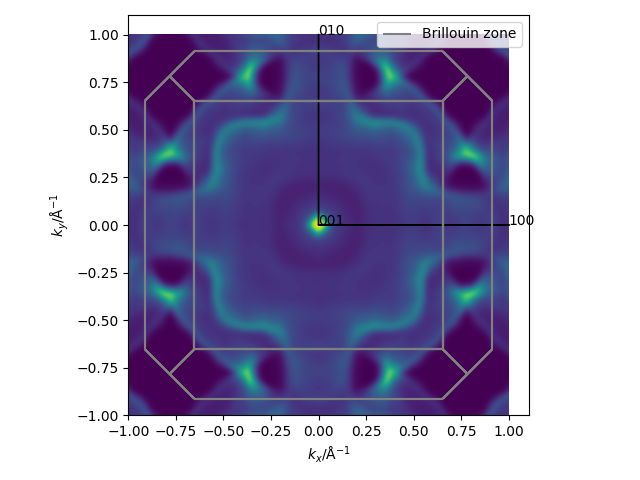
Projected Fermi surface

from fplore import FPLORun
from fplore.plot import plot_bz_proj
from fplore.util import cartesian_product
import matplotlib.pyplot as plt
import numpy as np

#run = FPLORun("../example_data/fermisurf") #yrs TODO fix fermisurf run
run = FPLORun("../example_data/yrs") #yrs

## limit to bands close to fermi level to reduce memory usage
#bands = run.band.bands_at_energy(e=0., tol=5*0.04)
#selected_energy_data = run.band.data['e'][..., bands]

ip = run.band.interpolator
axes = [np.linspace(-1, 1, 100)]*3
k_sample = cartesian_product(*axes)
data = ip(run.backfold_k(k_sample))

data = data.reshape(tuple(map(len, axes)) + (-1,))

# axis to project along, 0: x, 1: y, 2: z
axis_to_project = 2

visible_axes = [0, 1, 2]
visible_axes.remove(axis_to_project)

axis_labels = [r'$k_x / \mathrm{\AA}^{-1}$',
               r'$k_y / \mathrm{\AA}^{-1}$',
               r'$k_z / \mathrm{\AA}^{-1}$']

im = run.band.smooth_overlap(data, e=0, scale=0.04, axis=axis_to_project)
im = im.T  # so the first axis (x) is displayed horizontally not vertically

plt.imshow(im, extent=(axes[visible_axes[0]][0], axes[visible_axes[0]][-1],
                       axes[visible_axes[1]][0], axes[visible_axes[1]][-1]),
           interpolation="bicubic", origin='lower')
plot_bz_proj(run, plt.gca(), axis=axis_to_project, color='grey')

plt.xlabel(axis_labels[visible_axes[0]])
plt.ylabel(axis_labels[visible_axes[1]])
plt.legend()
plt.tight_layout()
plt.show()