Band projection

# sphinx_gallery_thumbnail_number = 2

import numpy as np
import matplotlib.pyplot as plt

from fplore import FPLORun
from fplore.plot import project, plot_bz
from fplore.util import sample_e, linspace_ng

run = FPLORun("../example_data/fermi")

point_1 = np.array((0.5, 0, 0))
point_2 = np.array((0.5, 0.5, 0))
point_3 = np.array((0, 0, 0.5))

level_indices = run.band.bands_within(-0.25, 0.25)
path = linspace_ng(point_1, point_2, point_3,
                   num=(50, 50))
path = run.fplo_to_k(path)

axes, idx_grid = run.band.reshape_gridded_data()
bands_to_sample = run.band.data['e'][..., level_indices]

grid_data = bands_to_sample[idx_grid]
bands_along_path = sample_e(axes, grid_data, path, order=2)
# bands_along_path = run.band.interpolator(path)

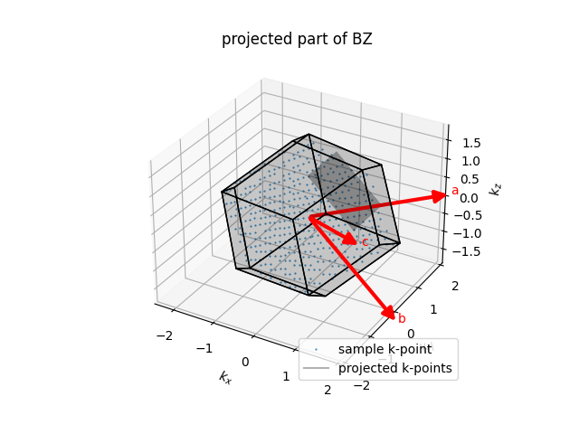
Illustration of the part of the Brillouin zone that is being projected.

f1 = plt.figure()
ax = f1.add_subplot(111, projection='3d')

points = path.reshape(-1, 3)
plot_bz(run, ax, k_points=True, high_symm_points=False, use_symmetry=True)
ax.plot(*points.T, color='k', alpha=0.3, label="projected k-points")

ax.set_title('projected part of BZ')
ax.legend(loc='lower right')

plt.show()

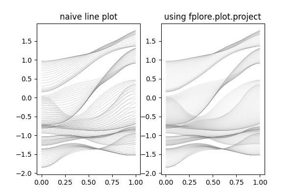
Projecting the bands.

f2 = plt.figure(figsize=(6, 4))
ax1 = f2.add_subplot(1, 2, 1)
ax2 = f2.add_subplot(1, 2, 2, sharex=ax1, sharey=ax1)

n_energy_levels = bands_along_path.shape[-1]
for i in range(n_energy_levels):
    bap = bands_along_path[..., i]
    i = np.linspace(0, 1, bap.shape[0])
    j = np.linspace(0, 1, bap.shape[1])
    ij = np.meshgrid(i, j, indexing='ij')
    ax1.plot(ij[0], bap, color='gray', lw=0.1)
ax1.set_title('naive line plot')

for i in range(n_energy_levels):
    bap = bands_along_path[..., i]
    i = np.linspace(0, 1, bap.shape[0])
    j = np.linspace(0, 1, bap.shape[1])
    i, j = np.meshgrid(i, j, indexing='ij')
    pc = project(i, j, bap, axis=1, color=(0.5, 0.5, 0.5, 1.0))
    ax2.add_collection(pc)
ax2.set_title('using fplore.plot.project')

plt.show()